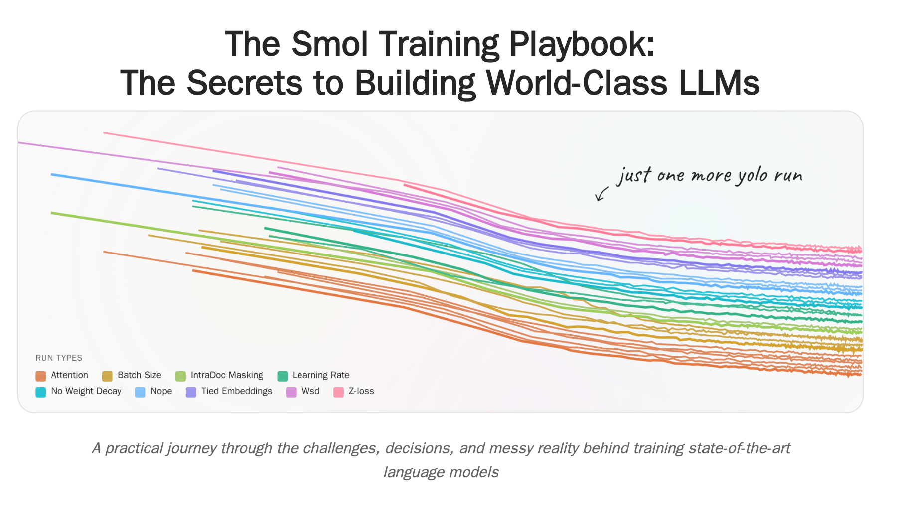
[Notes] The Smol Training Playbook

Ablations

Ablations - run experiments at a small scale and get results that we can confidently extrapolate to during the final production run.

• Two main approaches: (1) Take the target model size & train on fewer tokens. (2) If target model is too large, train a smaller proxy model for ablations
• The tricky part is that components often interact in non-linear ways - and we don’t have the time/compute to test everything out
• Start by testing promising changes against your current baseline. When something works, integrate it to create a new baseline, then test the next change against that
• Ablations can be more than half the cost of the main training run. So, ablation costs must be factored into your compute budget’s plan

Three common task formulations

• Multiple choice format (MCF): Requires model to select an option from a number of choices explicitly presented in the prompt
• Close formulation (CF): Requires model to fill in a blank; choices isn’t provided in the prompt
• Freeform generation (FG): Look at the accuracy of the greedy generation for a given prompt

FG requires a lot of latent knowledge in the model & is usually too difficult a task for models to be really useful in short pre-training ablations before a full training. So, we focus on MCF or CF when running small-sized ablations.

• Research has shown that models struggle with MCF early in training, only learning this skill after extensive training, making CF better for early signals
• Use CF for small ablations, and integrate MCF in the main run as it gives better mid-training signal once a model has passed a threshold

Attention Architecture

Multi-head attention (MHA) is the original attention introduced in transformers. We have N attention heads independently transforming the hidden state into queries, keys, and values, then using the current query to retrieve the most relevant token by match on the keys and finally forwarding the value associated with the matched tokens.

At inference time we don’t need to recompute the KV values for past tokens and can reuse them. The memory for past KV values is called the KV-Cache

Simple calculation to estimate KV-cache memory with MHA and seq len of 8192

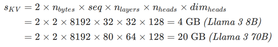
• Leading factor 2 comes from storing both key and value caches

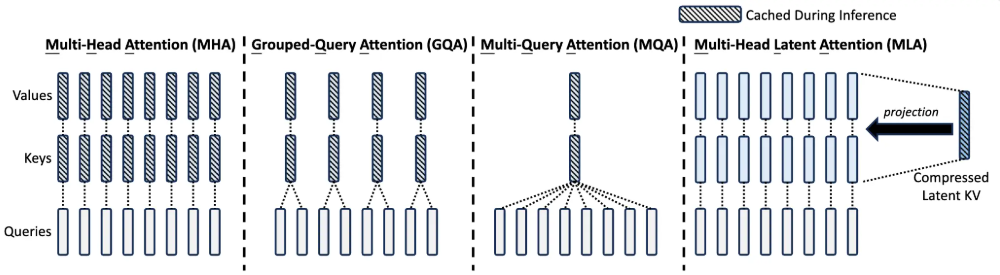
MQA, GQA, and MLA all reduce the number of distinct KV representations

• MHA: Separate Q, K, V projection matrices for each head of that decoder block
• Multi-query Attention (MQA): One K, V projection matrix shared by all query heads of that decoder block
• Grouped-query Attention (GQA): Heads are partitioned into groups of size H/G (H=no. of heads, G=no. of groups, G/H=no. of query heads per KV group). Query heads in the same group share the same K, V proj matrix
• Multi-latent Attention (MLA): KV vectors across all heads (not the w_K, w_V projection matrices) are compressed into small latent representations, and decompressed into full-dimensional KV values at runtime

These drastically reduce the KV cache memory usage

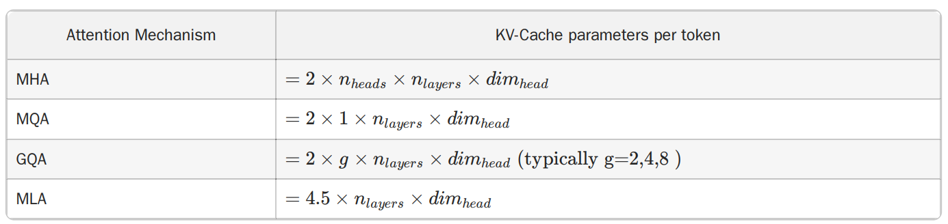
• In MHA, we store one KV value per token per head (so we must multiply by n_heads to get the total memory usage of that token), but for MLA we store one latent vector per token per layer (so we don’t have to multiply by n_heads)

Attention Masking

How we apply attention across our training sequences impacts both computational efficiency and model performance.

Intra-document masking: We use packing to fit variable-length docs into fixed-length training sequences - combining multiple shorter docs into a single seq. Intra-document masking ensures tokens can only attend to previous tokens within the same document. It’s found to give significant benefits for long-context extension.

Embedding sharing (tied embeddings): Instead of having 2 separate learned embeddings - input embedding, output embedding (final linear layer), reuse input embeddings in the output. Benefits SLMs, where embeddings constitute a large portion of total param count

Positional Encoding

• Absolute Position Embeddings (APE): Used by early transformers. Learned lookup tables that mapped each position to a vector that gets added to token embeddings. No out-of-the-box generalization capabilities to longer seqs
• Rotary Position Embedding (RoPE): Dominate recent LLMs. Rotate query and key vectors by angles that depend on their absolute positions, in a way that encodes their relative distance via dot product of their rotated representations
• No Position Embedding (NoPE): No explicit positional encoding; allow the model to implicitly learn positional info through causal masking & attention patterns. Better length generalization compared to RoPE, so it can handle longer context, but show weaker performance on short context reasoning compared to RoPE
• RNoPE Hybrid approach: Alternate between RoPE and NoPE. RoPE layers provide explicit positional information and handle local context with recency bias, while NoPE layers improve information retrieval across long distances.

Limiting Attention Scopes

Strategically restrict which tokens can attend to each other, keeping attention patterns within familiar ranges while still processing the full sequence.

• Chunked attention: Divide sequence into fixed size chunks; tokens can only attend within their chunk
• Sliding Window Attention (SWA): Based on intuition that most recent tokens are most relevant; each token attends only to the most recent N tokens
• Dual Chunk Attention (DCA): Extends chunked attention while maintaining cross chunk information flow. Intra chunk attention (attend within their chunk) + inter chunk attention (attend to previous chunks) + local window (preserve locality between neighbouring chunks)

Improving Training Stability

• Z-loss: Regularization technique that prevents final output logits from growing too large. Helps maintain numerical stability during training
• Remove weight decay: Weight decay causes embedding norms to gradually decrease during training, leading to larger gradients in early layers
• QK-Norm: Apply layer norm to both Q, K vectors before computing attention, preventing attention logits from becoming too large. QK-norm hurts long-context tasks

Deeper models (more layers) outperform equally sized (same param count) wider ones on language-modeling and compositional tasks until the benefit saturates. This “deep-and-thin” strategy works well for sub-billion-parameter LLMs in MobileLLM ablations, whereas wider models tend to offer faster inference thanks to greater parallelism.

MoE

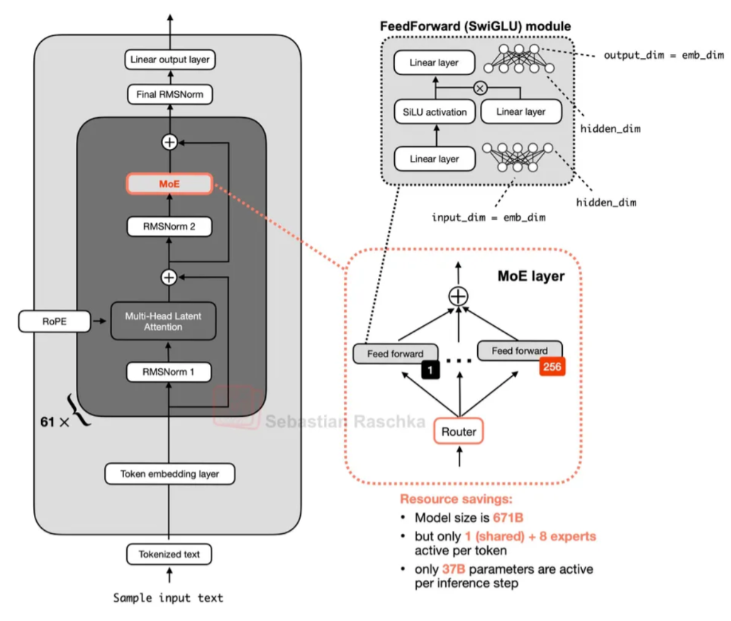
We replace the single MLP in the attention block with multiple MLPs (“experts”) and add a learnable router before the MLPs. For each token, the router selects a small subset of experts to execute.

• Routing happens per token, not per sequence! Different tokens in the same sequence can use different experts

Efficiency Leverage (EL): Measures how much dense compute you’d need to match the loss achieved by an MoE design. Higher EL = MoE configuration is delving more loss improvement per unit of compute (FLOPs) compared to dense training

Activation Ratio: What % of experts are activated per token

Sparsity: Higher sparsity = less experts activated per token. Sparsity = 1/activation_ratio. E.g. sparsity=4 means 1/4 of experts are activated per token.

• Holding the number and size of active experts fixed, increasing the total number of experts (i.e. lowering activation ratio / increasing sparsity) improves loss, with diminishing returns once sparsity gets very high

Granularity (G): No. of experts needed to match the dense MLP width

• Common rule of thumb in dense models is to have dimension of MLP set to d_intermediate = 4 * d_model (hidden dim)
• Granularity is how many experts it takes to match the dense MLP width.4d_model = d_intermediate = Gd_expert (expert dim)

Shared Experts: Route every token to a small set (1-2) of always-on experts. These shared experts absorb the basic, recurring patterns in the data so the remaining experts can specialize more aggressively.

Adding an auxiliary load-balancing loss to the router ensures it learns to route to each expert and doesn’t just use a handful of experts.

Hybrid Models

Recent trends include augmenting the standard dense/MoE architecture with state space models (SSM) or linear attention mechanisms, to deal efficiently with long context

• State space models: Replace attention with a hidden state that evolves over time. Its essentially RNNs where the hidden-state evolution is linear (rather than non-linear)
• Linear attention: Reorder computations so attention no longer costs O(n^2d) but O(T*d^2) - where T is seq len, d is head_dim. Reorder matmuls, never building a TxT attention matrix but instead having a global memory vector that’s updated overtime. Softmax is entirely removed

Comparing Base Architectures

• Dense transformers: Widely supported, stable training. Compute scales linearly with size
• MoE: Feed-forward layers replaced with multiple experts. Better performance per compute, but high memory usage as all experts must be loaded. Distributed training is a nightmare
• Hybrid: Combine transformers with SSMs, offering linear complexity for some ops vs attention’s quadratic scaling. Potentially better long-context handling but less mature resources than dense/MoE

Tokenizer

Vocab size

• Larger vocab = can include more whole words/subwords = fewer tokens per sentence = more efficient compression
• Computational trade-off: Vocab size affects the size of embedding matrices
• Compression gains from larger vocab size decrease exponentially - an optimal size exists
• Larger models benefit from bigger vocabularies as compression saves more on the forward pass than additional embedding tokens cost in softmax

Tokenizer quality evaluated using

• Fertility: Average no. of tokens needed to encode a word. Lower fertility = better compression = faster training/inference
• Proportion of continued words (PCW): What % of words are split into multiple pieces. Lower PCW = better since less words are fragmented

Likely need to train own tokenizer if we’re training for low-resource languages or have a very different data mixture.

Optimizer & Training Hyperparameters

Adam optimizer: in addition to looking at the gradients alone, we also consider how much the weights changed in the previous steps. This makes the learning rate for each parameter adapt based on the momentum.

• AdamW (Adam with weight decay) is the most widely used, decoupling weight decay from the gradient update

Learning rate schedules ensure that we have high learning rates at the start, and lower learning rates as we near convergence

• Cosine decay: Initial go-to. Downside is we need to know total training steps upfront since cosine cycle length must match total training duration
• Warmup-Stable-Decay (WSD): Maintain constant high learning rate for most of training and sharply decay in the final phase (e.g. last 10-20% of tokens)
• Multi-Step: Do discrete drops to decrease the learning rate (e.g. after 80% of training, 90% of training…)
• With WSD & Multi-Step, we can extend training mid-run without restarting - since they don’t depend on a fixed “end time”

Optimal learning rate depends on training duration, so the learning rate that converges fastest in a short ablation might not be the best one for the full run. We use scaling laws for this

Batch size: No. of samples processed before updating model weights

• Increasing BS improves throughput, but beyond a certain point it starts to hurt data efficiency has model needs more tokens to reach the same loss - this breakpoint is called critical batch size
• When batch size grows, each mini-batch gradient is a better estimate of the true gradient, so you can safely take a larger step (i.e., increase the learning rate) and reach a target loss in fewer updates
• Critical batch size isn’t fixed, it grows as training progresses. Batch size warmup will adjust the batch size as training continues

Scaling Laws can help us pick starting points for BS and LR - they establish empirical relationships describing how model performance evolves as we increase training scale, whether through larger models or more training data

• Training scale is quantified as compute budget (C), measured in FLOPs, approximated as: C = 6 * N * D, where N=no. of model params, D=no. of training tokens. 6 comes from estimates of how many floating-point ops are required per parameter per token
• We can derive scaling laws that predict optimal learning rates and batch sizes as functions of total compute budget (C). Plot LR/BS (y-axis) against the compute budget (x-axis)

As training becomes larger and longer, we want more stable updates (hence, smaller learning rates) and more efficient gradient estimation (hence, larger batch sizes)

Data Curation

Filtering out all the lower quality data and training on the highest quality data only would result in repeating data many times. This kind of repetition can be harmful, so we should ideally be able to make use of higher & lower quality data while still maximizing model performance.

In the early days, the standard approach was to fix a single data mixture for the entire training run. We’re shifting toward multi-stage training where the data mixture changes over the course of training.

• Motivation is that LLM’s final behavior is strongly influenced by data seen toward the end of training (annealing phase)
• Strategy: Upweigh more plentiful sources early in training and mix in smaller, higher quality sources towards the end

When testing data mixtures, try to run them at the target model scale. This is because small & large models have different capacities - running data ablations at too small a scale risks drawing the wrong conclusions about the optimal mix

• Automated approaches for finding optimal data proportions include: DoReMi, Rho Loss, RegMix

Extending Context

Research shows that extending context with a few dozen to a hundred billion tokens toward the end of training, or during continual pretraining, is enough to reach good long context performance.

Gradually extended context in stages, giving the model time to adapt at each length before pushing further. Sequential scaling: 4k→32k→64k

Post Training

Different frameworks offer different support, from supervised fine-tuning (SFT) to preference optimization (PO) and reinforcement learning (RL)

Most post-training pipelines begin with SFT as it’s cheap, stable (compared to RL which is sensitive to reward design & hyperparameters). It makes later methods like DPO/RLHF far more effective

When choosing a base model for post-training

• Model size: Larger models generalize better, and often with fewer samples
• Architecture: Dense models are simpler to fine-tune compared to MoE
• Track record: Good if base model has already spawned a collection of strong community-led post-trained models

Ensure the post-training chat template is compatible with the inference engine you intend to use. Some engines like vLLM/SGLang have dedicated parsers for reasoning & tools.

SFT Considerations

• Full finetuning or LoRA/QLoRA?
• Data parallelism (usually for small models) or use FSDP/ZeRO to shard model weights & optimizer states (for larger models). Context parallelism (split seq dim across GPUs) for long context
• Kernels like FlashAttention or Liger drastically lower vRAM usage
• Mask loss to train only on assistant tokens, ignoring user/system msgs. If we train the model to predict all tokens, it effectively learns to autocomplete user queries, rather than focusing on producing high-quality assistant responses.
• Packing concatenates multiple sequences together, reducing no. of padding tokens that waste compute. For smaller/diverse datasets, might be better to disable packing to preserve granularity & ensure every example contributes cleanly to optimisation
• Learning rate: Optimal LR in SFT is typically an order of magnitude smaller than the one used during pretraining. Aggressive update can lead to catastrophic forgetting

Continual pretraining (mid-training) involves taking a base-model & training it further on large amounts of domain-specific tokens before doing SFT. This shifts the model toward a distribution that better supports the capabilities you care about

• Starting SFT from a model that has already integrated that core skill allows your model to better focus on the specific topics in your SFT data
• In practice, you’ll often iterate: run SFT to identify weak areas, then do targeted mid-training, then run SFT again.

In SFT, the model has no clear signal for what counts as “better”. In preference optimization (PO), we give the model comparative feedback like response A is better than response B”. These preferences provide a more direct training signal for quality

• Two ways to create preference datasets: (a) Strong vs weak - same prompt passed to a weaker & stronger-performing model - labelled as rejected/chosen respectively. (b) On-policy grading: Same model generates multiple candidates, then use an external grader (verifier/reward model) to score responses
• Direct Preference Optimization (DPO) is the first PO algorithm.
• Alternatives include (a) Kahneman-Tversky Optimization (KTO) which relies on individual responses being desirable or not (e.g. based on 👍 or 👎 from users) rather than preference pairs, (b) Odds Ratio Preference Optimization (ORPO) which integrates preference optimization directly into SFT via an odds ratio in cross-entropy loss, removing the need for separate PO stage, (c) Anchored Preference Optimization (APO) which explicitly regularizes how much model’s likelihoods for chosen/rejected outputs should shift

Typically 3 hyperparameters for PO

• Learning rate, typically a factor of 10-100x smaller than the one used for SFT.
• The β parameter, which controls the size of the margin between preference pairs. Lower values of beta encourage staying close to the original model while higher values allow the model to match the preference data more closely
• The batch size

PO is only as good as the offline preference data we collect. We can use on-policy and RL-based methods to generate fresh training feedback online.

Instead of supervising the model with preferences, you let it interact with an environment (e.g. math verifier, a code executor, or even real user feedback), and learn directly from the outcomes. RL shines when we can check correctness automatically (have a high quality verifier/reward model, etc.), we require multi-step reasoning or planning )which local preferences can’t capture), or we want to optimize for objectives beyond preference labels.

2 main flavors of RL

• Reinforcement Learning from Human Feedback (RLHF): Human annotators compare model outputs (e.g. “A is better than B”) and a reward model is trained to predict those preferences. The policy is then fine-tuned with RL to maximise the learned reward.
• Reinforcement Learning with Verifiable Rewards (RLVR): Involve use of verifiers that check whether a model’s output meets some clearly defined correctness criteria (e.g. does the code compile and pass all tests, or is the mathematical answer correct?). The policy is then fine-tuned with RL to produce more verifiably-correct outputs.

The efficiency and stability of RL-based training depends heavily on whether the learning algorithm is on-policy or off-policy.

• On-policy: Trains the model using data generated by its current policy. Methods such as GRPO typically fall into the category of on-policy optimisation algorithms, where the model (the policy) that generates the completions is the same as the one being optimised.
• Off-policy: Trains the model using data generated by a different (often older/external) policy, reusing fixed datasets

Other approaches to on-policy learning include

• Online DPO: Rather than training once on a fixed preference dataset, the model continually samples new responses, collects fresh preference labels (from reward models or LLM graders), and updates itself
• On-policy distillation: Instead of preferences, the signal comes from a stronger teacher model. The student samples responses at every training step and the KL divergence between the student and teacher logits on these samples provides the learning signal

Choose which method based on

• Online DPO: You can get preference labels cheaply. Best for aligning behaviour with evolving distributions.
• On-policy Distillation: You have access to a stronger teacher model and want to transfer capabilities efficiently.
• Reinforcement Learning: Best when you have verifiable rewards or tasks requiring multi-step reasoning/planning. Can be used with reward models, but there are challenges like reward-hacking, where the model takes advantage of weaknesses in the reward model.

In on-policy RL, for each prompt we usually get multiple different completions (rollouts), score each completion with a reward model or verifier, and then use all of them together to compute a policy update.

For small models, on-policy distillation typically outperforms RL-based methods (i.e. GRPO) at a fraction of the compute cost, because instead of generating multiple rollouts per prompt, we only sample one, which is then graded by the teacher in a single forward-backward pass.

A weakness of on-policy distillation is that the teacher and student must share the same tokenizer. General OnPolicy Logit Distillation (GOLD) allows any teacher to be distilled into any student.

Infrastructure

At the highest level, a GPU performs 2 essential tasks

1. Move and store data (memory system)
2. Do useful work with the data (compute pipelines)

GPUs measure performance in FLOPs (floating-point ops per second). Real-world performance is 70-77% of theoretical peaks due to memory bottlenecks. Theoretical peaks represent max computational throughput when all compute units are fully utilized & data is readily available.

The fundamental building blocks of GPU compute are Streaming Multiprocessors (SMs), independent processing units that execute instructions in parallel. Each SM contains two types of cores: CUDA cores for standard floating-point operations, and specialized Tensor Cores optimized for matrix multiplication, which dominate deep learning tasks.

Training efficiency is captured by Model FLOPs Utilization (MFU): the ratio of useful model computation to theoretical peak hardware performance. Much of the gap comes from inter-node communication overhead in distributed training.

Besides choosing the right kernel API, we also need to ensure those kernels are compiled for the right hardware generation. Compute Capability (CC) is NVIDIA’s versioning system that determines which instructions and features your GPU supports. Kernels compiled for a specific compute capability may not run on older hardware, and you might miss optimizations if your code isn’t compiled for your target GPU’s CC.

Modern AI is often memory-bound. Operator fusion (like Flash Attention) achieves 2-4× speedups by keeping intermediate results in fast on-chip memory instead of writing to slow HBM

• For optimal performance, aim to minimize traffic to slower memory tiers (HBM) while maximizing utilization of faster tiers (shared memory, registers).

Moving up the hierarchy toward the compute units, we find progressively faster but smaller memory tiers

• L2 cache : A large SRAM-based cache shared across the GPU, typically several tens of megabytes
• L1 cache and Shared Memory (SMEM) : Each Streaming Multiprocessor (SM) has its own L1 cache and programmer-managed shared memory, which share the same physical SRAM storage
• Register File (RMEM) : At the top of the hierarchy, registers are the fastest storage, located directly next to compute units. Registers are private to individual threads

Understanding whether your kernel is compute-bound or memory-bound determines which optimizations will help.

• If you’re memory-bound (spending most time moving data), increasing compute throughput won’t help: You need to reduce memory traffic through techniques like operator fusion
• If you’re compute-bound (spending most time on FLOPs), optimizing memory access patterns won’t help: You need more compute power or better algorithms

There are 4 critical communication links in GPUs

• GPU-CPU: How the CPU schedules work and transfers data to GPUs. There is kernel launch overhead (when CPU launches kernels), which can be reduced via CUDA Graphs which reduce overhead by batch operations. How fast the CPU can communicate with GPU is determined by the PCIe connection between them. NUMA affinity tries to make GPU processes run on CPUs with the same socket
• GPU-GPU intra-node: How GPUs on the same machine communicate. GPUDirect RDMA enables direct communication between GPUs by allowing direct access to GPU memory. NVLink is Nvidia’s high-speed GPU-to-GPU interconnect technology
• GPU-GPU inter-node: How GPUs across different machines communicate over the network. Use high-speed networks like InfiniBand or RoCE
• GPU-Storage: How data flows from external storage to GPU memory. During training, GPUs need to continuously read data from storage and write model states back. I/O operations can become bottlenecks if not properly optimized. GPUDirect Storage (GDS) enables a direct data path between storage path & GPU memory. Other storage tech include RAID, NVMe, WekaFS, FSx Lustre

Building Resilient Training Systems

During training, we track key metrics across all nodes such as GPU temperatures, memory usage, compute utilization and throughput fluctuations. We use Prometheus to collect DCGM metrics from all GPUs and visualize them in Grafana dashboards for real-time monitoring.

Marketing specs assume perfect cooling, but reality is messier. GPUs automatically reduce clock speeds when they overheat, cutting performance below theoretical maximums even in well-designed systems.

In distributed training, you’re only as fast as your slowest node. Thermal throttling doesn’t just hurt the affected GPU; it cascades across your entire distributed training setup. A single node with thermal throttling becomes the bottleneck.

Your model can fail mid-training. Try to automate your resume process. On Slurm, for example, you can just use SBATCH --requeue so the job restarts automatically from the latest checkpoint

• Checkpoint saving should happen in the background without impacting training throughput
• Storage usage can skyrocket if you store every checkpoint… you can just store the most recent checkpoint instead

Running evaluations manually becomes a bottleneck fast. LightEval automatically runs evaluations on checkpoints. Every saved checkpoint triggers an evaluation job on the cluster.

Optimizing training Throughput

Get the no. of GPUs needed via:

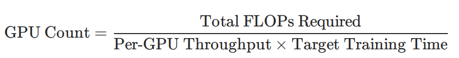
• Total FLOPs Required: The computational work needed to train your model (depends on model size, training tokens, and architecture)
• Per-GPU Throughput: How many FLOPs per second each GPU can actually deliver (not theoretical peak)
• Target Training Time: How long you’re willing to wait for training to complete

Adding more GPUs can actually make training slower - Amdahl’s Law. The speedup from parallelization is fundamentally limited by the serial (non-parallelizable) portion of your workload. In LLM training, this “serial” portion is primarily communication overhead: the time spent synchronizing gradients, weights, activations across GPUs that can’t be parallelized away.

Parallelism that reduces per-GPU memory footprint includes Tensor Parallelism (split model layers across GPUs), Pipeline Parallelism (split model depth across GPUs), or ZeRO optimizer sharding (distribute optimizer states)